Quick Start

Aims for this tutorial:

• calculate a synthetic spectrum;

• convolve with Gaussian functions of varying full-width-at-half-maximum (FWHM);

• visualize results.

Spectral synthesis from the command line

Short story

Here is the full command sequence:

mkdir mystar
cd mystar
copy-star.py
link.py
run4.py
plot-spectra.py --ovl flux.norm flux.norm.nulbad.0.120

Long story

Create a new directory

mkdir mystar
cd mystar

Gather input data

Input data consists of:

1. stellar parameters (temperature, chemical abundances etc.) and running settings (e.g., calculation wavelength interval);

2. star-independent physical data: line lists, atmospheric model grid, partition functions etc. that are less likely to be modified. We refer to these as “common” data.

Stellar data and running settings

The following displays a menu allowing you to choose among a few stars:

copy-star.py

After running this, the following files will be copied into the “mystar” directory:

• “main.dat”: main configuration (editable with mained.py, x.py)

• “abonds.dat”: chemical abundances (editable with abed.py, x.py)

Common data

For these data, we will create links instead of copying the files, as the files are big and/or unlikely to change:

link.py

The following links should appear in your directory now:

• absoru2.dat

• atoms.dat

• grid.mod

• grid.moo

• hmap.dat

• molecules.dat

• partit.dat

Spectral synthesis pipeline

Spectral synthesis involves a few steps, as shown in Figure 1, and described in the next subsections.

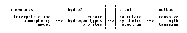
Figure 1 – PFANT spectral synthesis pipeline showing the Fortran program names and what they do.

Interpolate the stellar atmospheric model

This step takes a 3D grid of atmospheric models (usually a file named “grid.mod”) and interpolates a new model given a certain point (temperature, gravity, metallicity) (specified in the main configuration file) contained within the limits of the grid.

innewmarcs

will create two files: “modeles.mod” and “modeles.opa”.

Note

If the combination of (temperature, gravity, metallicity) is outside the limits of the grid (e.g., if you choose star Mu-Leo), innewmarcs will refuse to interpolate. However, it can be forced to use the nearest points in the grid with:

innewmarcs --allow T

Create hydrogen lines profiles

hydro2

will create files such as: “thalpha” (Figure 12), “thbeta”, “thgamma” etc.

Calculate synthetic spectrum

pfant

creates files:

1. “flux.spec”: spectrum

2. “flux.cont”: continuum

3. “flux.norm”: normalized spectrum ((1) divided by (2))

To visualize these files:

plot-spectra.py flux.spec flux.cont flux.norm

will open a plot window (Figure 2).

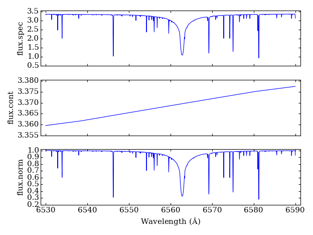
Figure 2 – plots of three files generated by pfant.

Convolve synthetic spectrum with Gaussian function

The following will take the normalized spectrum from the previous step and convolve it with a Gaussian function of FWHM = 0.12, creating file “flux.norm.nulbad.0.120”:

nulbad --fwhm 0.12

Plot spectra

plot-spectra.py --ovl flux.norm flux.norm.nulbad.0.120

opens a plot window where one can see how the spectrum looks before and after the convolution (Figure 3).

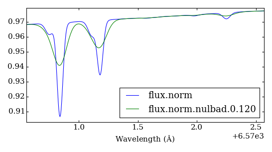
Figure 3 – plot comparing spectra without and after convolution with Gaussian function (FWHM = 0.12)

Running the four calculation steps at once

The script run4.py is provided for convenience and will run all Fortran binaries in sequence.

run4.py --fwhm 0.12

Hint

The same command-line options available in the Fortran binaries are available in run4.py.

Spectral synthesis using the Graphical interface

Alternatively to the command line, you can use the “PFANT Launcher” (x.py) provided by the F311 project.

First it is necessary to create a new directory and gather the input data (as in the spectral synthesis from the command line above):

mkdir mystar
cd mystar
copy-star.py
link.py

Now you can invoke the “PFANT Launcher” application (Figure Figure 4):

x.py

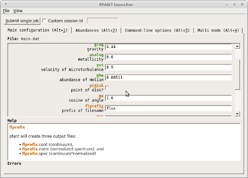
Figure 4 – Screenshot of the x.py application

Here is a suggested roadmap:

1. Change parameters in Tab 1/2/3 (Tab 4 is a different story)

2. Click on the “Submit single job” button: a new window named “Runnables Manager” opens

3. When the “Status” column shows “nulbad finished”, double-click on the table item: “PFANT Explorer” window opens

4. Double-click on “flux.norm”: turns green (if wasn’t so)

5. Double-click on “Plot spectrum”: spectrum appears

Writing Python scripts with package pyfant

Python package "pyfant provides an API that allows one to perform spectral synthesis from Python code, manipulate PFANT-related data files, and more.

Here is a simple spectral synthesis example. The following code runs the Fortran binaries (innewmarcs, hydro2, pfant, nulbad) in a way that is transparent to the Python coder, and then plots resulting synthetic spectra (Figure 5):

import pyfant
import f311
obj = pyfant.Combo()
obj.run()
obj.load_result()

# Plots continuum, spectrum, normalized in three sub-plots
f311.plot_spectra_stacked([obj.result["cont"],
                           obj.result["spec"],
                           obj.result["norm"]])

# Plots normalized unconvolved, normalized convolved spectra overlapped
f311.plot_spectra_overlapped([obj.result["norm"],
                              obj.result["convolved"]])

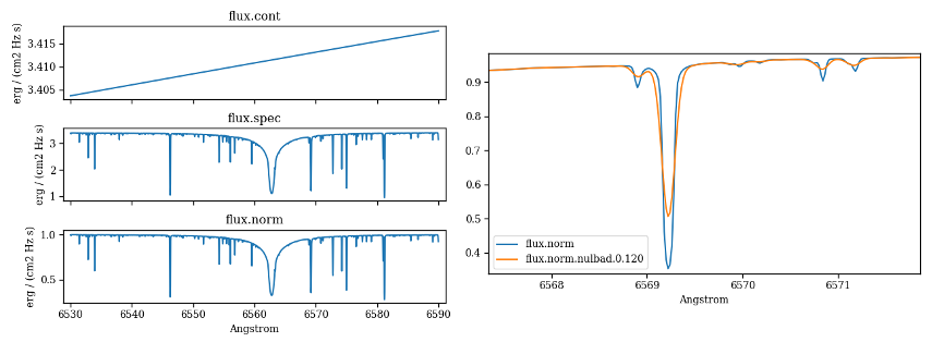
Figure 5 – Plots generated from code above.

More Python examples can be found at https://trevisanj.github.io/pyfant